Longitudinal Electrodynamics and Scalar Waves

This thread starts on solid ground and reaches a long way. The ground is mathematics from 1903 that is still taught. Above it sit measured effects that surprise people the first time they meet them, and above those sit proposals nobody has measured yet. This chapter climbs that stack from the bottom.

The real mathematics: Whittaker's potentials

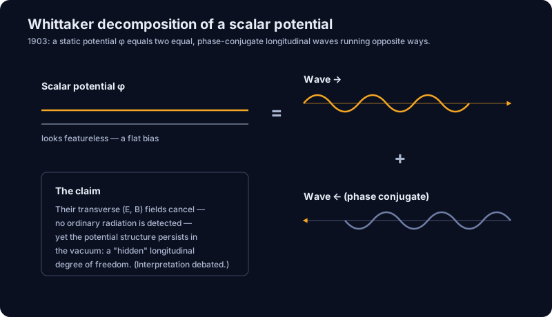
In 1903 and 1904 the mathematician E. T. Whittaker published two short papers. He showed that any solution of the relevant field equations can be written using just two scalar potential functions, and that a scalar potential splits neatly into a pair of waves running opposite ways. This is correct, lasting mathematics: the ancestor of the Debye potentials and Hertz vectors in textbooks like Stratton's. Physicists use it every day.

Whittaker's two-potential representation(10.1)

$$\mathbf{E},\mathbf{B} \;\longleftarrow\; \{\,\phi_1,\phi_2\,\}$$

Where potentials genuinely matter: Aharonov–Bohm

You often hear that potentials are more fundamental than fields. Mainstream physics agrees, in one precise and beautiful place: the Aharonov–Bohm effect, predicted in 1959 and confirmed by Tonomura's team in 1986. An electron travels where the magnetic field is exactly zero. It still picks up a measurable shift in its quantum phase, set by the potential alone.

It is measured, quantised and reproducible, and it anchors the whole vector-potential thread on this site. A potential can act on matter where no force acts.

Here is that experiment as an instrument. The shaded corridor is field-free: the magnetic field on the electron paths is zero at every setting, and the only thing you can change is the flux the two paths enclose between them. Dial it, and the fringes move — one whole fringe for every flux quantum, and back to where they started at the next one.

The interferometer with the field switched off

Split an electron beam, send the two halves either side of a magnetic flux that is completely confined and completely shielded, and bring them back together. On the paths themselves the magnetic field is exactly zero — the shaded corridor below is field-free the whole way. The vector potential there is not zero, and the fringes move. Dial the enclosed flux and watch the pattern slide sideways by exactly one fringe for every flux quantum.

• Upper path
• Lower path
• Confined flux

The enclosed flux

Enclosed flux, in flux quanta h/e

0.00

Advance by one whole flux quantumReturn to zero enclosed flux

What is happening: The enclosed flux is a whole number of quanta, so the phase difference is a whole number of turns and the pattern sits exactly where it started. This is the periodicity that makes the effect a measurement rather than a drift.

Magnetic field on the electron paths

zero, at every setting

Vector potential on the paths

zero, because no flux is enclosed

Phase difference between the two halves

0.00 radians

Fringe shift

0.00 fringe widths

The precision rule this instrument exists to protect: the vector potential controls phase. No energy is stored in it, and none needs to be — the phase difference is set by the flux the two paths enclose between them, which is exactly the quantity you are dialling.

Tonomura's 1986 experiment answered the obvious objection by construction: the flux sat inside a toroidal magnet wrapped in a superconducting shield, so stray field was not merely small on the electron wave but excluded from it. The shift was still there, and it was still one fringe per flux quantum.

Settled physics. Scope: a drawn two-path interferometer with a perfectly confined flux, which is the geometry of the published experiment. Beam energy, path length and magnet size are not modelled, and no absolute intensity is asserted. Φ₀ = h/e ≈ 4.136e-15 Wb.

The source sheet: Tonomura et al. 1986, Evidence for Aharonov–Bohm effect with magnetic field completely shielded from electron wave

What Maxwell already permits

Longitudinal fields — fields pointing along the direction of travel — are not exotic. Maxwell's equations give you them in three familiar places.

• The near field. Within about a wavelength of an antenna, the field has a component along the direction of travel. Every antenna engineer works with it. It stays bound to the source instead of radiating away.
• Plasmas. A plasma carries Langmuir waves. The electrons slosh back and forth along the direction of travel, the way sound moves through air. These are everyday, measured longitudinal waves.
• Guided surfaces. A Zenneck surface wave runs along the boundary between air and a lossy conductor such as ground or seawater. It carries a field component along its direction of travel and clings to the surface instead of spreading into space.

That is generous ground. Longitudinal electric fields exist, they carry energy where they are bound or guided, and engineers build with them already.

Free space is the harder case. In quantum electrodynamics the photon's longitudinal and timelike polarisations are bookkeeping modes, and the Gupta–Bleuler formalism cancels them out of free radiation. So a free-space longitudinal wave carrying energy would be new physics, not a corollary of Whittaker. The guided cases are the obvious place to hunt for something engineerable.

The proposals: scalar interferometry and the MEG

The modern thread runs through Tom Bearden and is repeated in independent-researcher streams. He argued that two beams can be arranged so their interference draws energy from the vacuum, and that the motionless electromagnetic generator (MEG, US6362718B1) already does it. The patent is public and the claims are there to read.

The test is clean and cheap. Poynting's theorem is the energy ledger of any electromagnetic device. Power out equals power in, minus what the fields store, minus what the device dissipates. Meter every input line on a bench and the ledger either closes or it does not. No independent laboratory has published that measurement yet.

Open question: does any scalar device close its energy ledger? What to watch next: a metered bench test of the MEG, published with the raw traces.

Speculative Free-space longitudinal energy transport, and Bearden-style vacuum tapping, are well-posed claims with named experiments and no measurement yet.

The objection

“Whittaker showed that scalar potentials underlie the fields, and the Aharonov–Bohm effect shows potentials are real where fields vanish. So longitudinal scalar energy waves should be real too.”

The answer

Both premises are correct, and this chapter teaches them as Definitive. The step that still needs work is the one from a bounded, measured phase effect to energy carried across empty space. In quantum electrodynamics the longitudinal and timelike photon modes are bookkeeping, and Gupta–Bleuler cancels them out of free radiation. Where longitudinal fields do carry energy is the near field, the plasma and the guided surface wave — all three engineerable today, and the more promising place to push. Watch for a controlled detection of a longitudinal wave carrying energy across a vacuum gap, or a metered bench test with the ledger closed. Whittaker stays Definitive and the free-space claim stays Speculative until one of those lands.

What the field added — July to September 2026

The vector potential had its season. Charles Chase, late of Lockheed's Skunk Works, described the A potential as more fundamental than the fields. It can change the phase of matter waves with no energy exchange. That is the Aharonov–Bohm effect this chapter already teaches. Chase described a coherent matter-wave beam built on that principle. Froning and Barrett's 1997 work on "conditioned" fields was read on screen. A beam's symmetry is raised from ordinary U(1) to SU(2), and the field gains structure that ordinary radiation lacks. It is now in the sources as the framework for engineering such fields. The aether returned in two forms. One was the historical case, told through Ørsted, Faraday, Maxwell and Hertz. The other was a citizen-science vertical interferometer, worth repeating on a controlled bench. Dirac's 1951 "Is there an Æther?" gave the question its most distinguished voice. Research log. For the full story of the vector potential — from a flow map anyone can picture to the matter-wave beam — take the vector-potential drill-down course.

Froning's own book added a geometry worth remembering. Before his group conditioned any beam, they asked a prior question: could the local density of the zero-point field be changed at all? Froning reports that it could. The hardware was a wound toroid deliberately built out of round — "instead of making a perfect donut, they made it like a triangle on one end, a teardrop shape." Only after that did they polarise and twist the beam into what the programme called a gravity beam. The order matters. The asymmetry came first, and it was a shape you could machine. What to watch: one of the more buildable things in this chapter.

---

Where each claim stands

• Whittaker's two-scalar-potential decompositions are valid mathematics. Definitive
• Potentials have real, bounded effects where fields vanish (Aharonov–Bohm). Definitive
• Longitudinal fields are real in the near field, in plasmas and on guided surfaces. Strong
• Free-space, energy-carrying longitudinal waves exist. Speculative
• Scalar interferometry draws usable energy from the vacuum. Speculative
• What would settle it: a controlled detection of a longitudinal wave carrying energy across a vacuum gap; and, for the devices, a metered bench test with the Poynting ledger closed. Both are bench-scale.

Sources

One Definitive mathematical node, one measured quantum effect, real guided longitudinal waves, and proposals with named tests.

Primary - the mathematics

• E. T. Whittaker (1903), "On the partial differential equations of mathematical physics," Math. Ann. 57, 333. DOI 10.1007/BF01444290.
• E. T. Whittaker (1904), "On an expression of the electromagnetic field due to electrons by means of two scalar potential functions," Proc. London Math. Soc. s2-1, 367 - the ancestor of the Debye potentials.
• J. Stratton, Electromagnetic Theory (1941) - the Debye and Hertz-vector descendants; standard working practice.

The measured anchor (beyond the source corpus)

• Y. Aharonov & D. Bohm (1959), "Significance of electromagnetic potentials in the quantum theory," Phys. Rev. 115, 485 - potentials act where fields vanish; confirmed by Tonomura et al. (1986).
• QED (Gupta-Bleuler): the photon's longitudinal and timelike polarizations are bookkeeping modes that cancel from free radiation. Real longitudinal modes live in the near field, in plasmas (Langmuir waves) and in guided surface waves.

Where the physics is worked out

• Bearden-style "scalar electromagnetics" (e.g. the MEG, US6362718B1) - a public patent with a specific claim. Poynting's theorem decides it: a metered bench test with every input line accounted for.
• H. D. Froning, Faster Than Light - the wound toroid built deliberately out of round (a teardrop rather than a perfect donut) used to change the local zero-point density before the beam was conditioned; read on air in the D. Miller ZPE All Stars interview, Hard Truths Podcast (8 September 2026; YouTube 5MIGis0S8Fc, @1:26:42-@1:27:36).

Where the replication stands: much of this thread is self-published, and the bench measurement above has not been made by an independent group. Whittaker is the Definitive node; the near-field, plasma and guided longitudinal waves are the Strong ground beneath it.