Tensor calculus and differential geometry
Learn to calculate geometry without confusing coordinates with physical structure.
Develop manifolds, tensors, metrics, covariant derivatives, geodesics, curvature, differential forms, and invariant diagnostics as the mathematical prerequisite for general relativity and metric-engineering analysis.
Before you begin
- • Calculus, vectors, and differential equations
- • Lagrangian mechanics
- • Linear algebra and multivariable calculus
By the end, you can
- • Transform vectors, covectors, and tensors between coordinate charts.
- • Compute Levi-Civita connections and geodesics from a metric.
- • Calculate curvature tensors and invariant contractions.
- • Separate coordinate effects from measurable geometric effects.
Interactive model
Explore before calculating
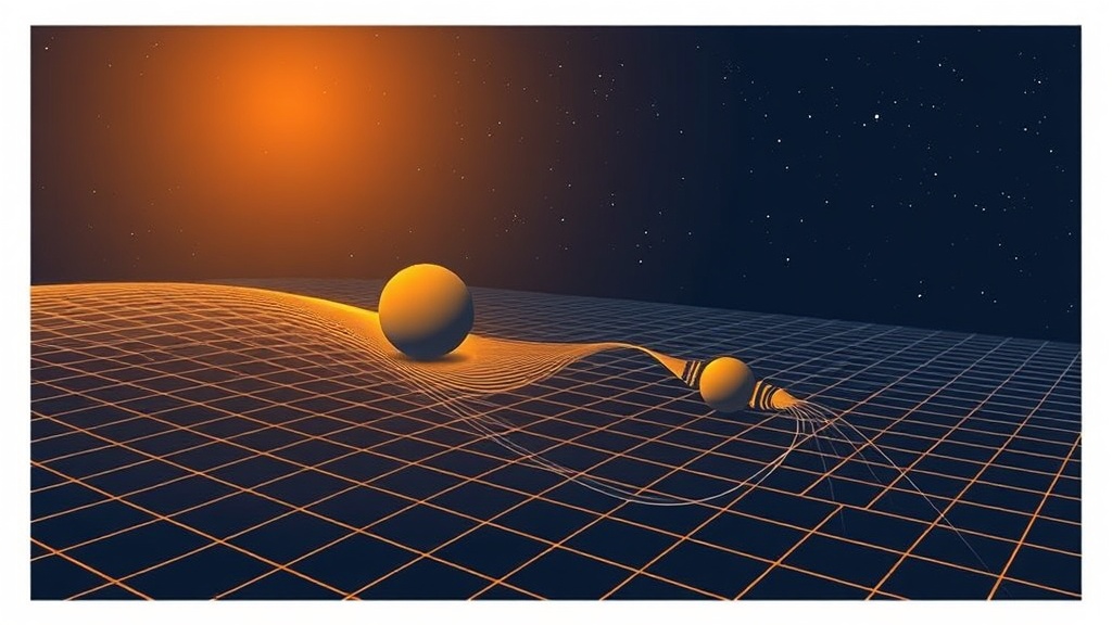
Live laboratory
Great-circle geodesic comparator
Compare the shortest surface path with a constant-latitude route. The difference makes intrinsic geometry visible without relying on an embedding analogy alone.
Difference: 404.7 km. Great-circle central angle: 60.00°.
Level 4 · Advanced undergraduate teaching kit
Record the investigation. Teach the reasoning.
A learner-facing lab record and a course-specific instructor guide turn the live model into a repeatable classroom investigation.
Learner record
Geodesic coordinate-invariance audit
Which features of a computed trajectory reflect geometry, and which reflect the chosen coordinate chart?
Download learner recordInstructor guide
Teach for evidence, not button pushing
Learners separate coordinate descriptions from invariant geometric and numerical statements in a geodesic calculation.
Download instructor guideLesson 1 of 3
Charts, tangent spaces, and tensors
Which quantities change with coordinates, and which geometric statements survive every chart?
A manifold is locally coordinatized but is not identical to any one coordinate grid. Tangent vectors act as directional derivatives, covectors act on vectors, and tensors are multilinear maps with a definite transformation law.
The metric is a symmetric nondegenerate rank-two tensor. It converts vectors to covectors, defines intervals and angles, and supplies a volume element once a signature and orientation are chosen.
Worked example
Transform the Euclidean plane metric from Cartesian to polar coordinates.
- 1. Write x=r cosφ and y=r sinφ.
- 2. Differentiate to obtain dx and dy.
- 3. Insert them into ds²=dx²+dy².
- 4. Collect dr², dr dφ, and dφ² terms.
ds²=dr²+r²dφ²; the geometry is flat even though the metric components vary.
Try it
Coordinate-versus-curvature audit
Materials: Symbolic notebook or paper
- 1. Write the plane metric in Cartesian and polar charts.
- 2. Compare component derivatives.
- 3. Compute or look up the scalar curvature.
- 4. Explain why varying components do not imply curvature.
Notice: A coordinate grid can bend on the page while invariant curvature remains zero.
Check your understanding: Can one decide whether a space is curved by inspecting whether metric components vary?
Answer: No.
Component variation can be caused by coordinates; curvature requires an invariant calculation such as the Riemann tensor.
Lesson 2 of 3
Connections, parallel transport, and geodesics
How can derivatives compare vectors that live in different tangent spaces?
A connection corrects ordinary component derivatives so the result transforms tensorially. The torsion-free, metric-compatible Levi-Civita connection is determined by the metric through Christoffel symbols.
Geodesics parallel-transport their own tangent. They are locally extremal paths for the interval under standard conditions, but coordinate acceleration along them need not vanish.
Worked example
Find the nonzero polar-plane Christoffel symbols.
- 1. Use g_rr=1 and g_φφ=r².
- 2. Evaluate Γᵃ_bc=½gᵃᵈ(∂_b g_dc+∂_c g_db−∂_d g_bc).
- 3. Only radial derivatives of r² survive.
- 4. Apply symmetry in the lower indices.
Γʳ_φφ=−r and Γᵠ_rφ=Γᵠ_φr=1/r.
Try it
Geodesics on a sphere
Materials: Globe, thread, and notebook
- 1. Stretch thread between two points along a great circle.
- 2. Compare with a line of latitude.
- 3. Write the spherical metric.
- 4. Identify which path is locally geodesic.
Notice: A geodesic is intrinsic to the surface and need not look straight in an embedding space.
Check your understanding: Are Christoffel symbols tensor components?
Answer: No.
Their inhomogeneous transformation term is exactly what repairs derivatives into covariant derivatives.
Lesson 3 of 3
Curvature, invariants, and differential forms
What measurement distinguishes true curvature from coordinate artifacts?
The Riemann tensor measures the failure of covariant derivatives to commute and the path dependence of parallel transport. Its contractions give the Ricci tensor and scalar curvature.
Differential forms package integration, orientation, and conservation cleanly. Exterior differentiation is coordinate-independent and Stokes' theorem unifies gradient, curl, divergence, and boundary laws.
Worked example
What curvature test distinguishes polar coordinates on a plane from a sphere?
- 1. Compute a curvature invariant rather than component derivatives.
- 2. For the plane, R=0.
- 3. For a sphere of radius a, Gaussian curvature is 1/a².
- 4. Conclude the spaces are intrinsically different.
Coordinate singularities can occur in flat space; nonzero curvature invariants cannot be transformed away.
Try it
Parallel-transport holonomy
Materials: Globe and arrow cutout
- 1. Carry the arrow north along one meridian.
- 2. Move along the equator.
- 3. Return along another meridian.
- 4. Compare final and initial orientation.
Notice: The rotation after a closed loop records integrated curvature.
Check your understanding: Why is the Ricci scalar alone insufficient to characterize all curvature?
Answer: Different Riemann tensors can share the same scalar contraction.
One scalar discards directional and tidal information.
Formula-to-meaning deck
Read the equation in ordinary language.
ds²=g_μν dx^μdx^ν
The metric turns coordinate displacements into an invariant interval.
Γ^ρ_μν=½g^ρσ(∂_μg_σν+∂_νg_σμ−∂_σg_μν)
The Levi-Civita connection is built from first derivatives of the metric.
R^ρ_σμν=∂_μΓ^ρ_νσ−∂_νΓ^ρ_μσ+Γ^ρ_μλΓ^λ_νσ−Γ^ρ_νλΓ^λ_μσ
Curvature records the noncommutativity of covariant transport.
Independent practice
Problem set
Work each problem before opening its hint and solution.
1. Compute the inverse and determinant of diag(−1,a²,b²,c²).
Reveal hint
Invert each diagonal element and multiply the diagonal for the determinant.
Reveal solution
g^{μν}=diag(−1,a⁻²,b⁻²,c⁻²), det g=−a²b²c².
2. Show that a constant metric in Cartesian coordinates has vanishing Levi-Civita connection.
Reveal hint
Every term in Γ contains a metric derivative.
Reveal solution
All ∂g terms vanish, so Γ^ρ_μν=0 in that chart.
3. A two-sphere has R=2/a². What happens as a→∞?
Reveal hint
Consider the local large-radius limit.
Reveal solution
R→0; a sufficiently small patch approaches a flat plane.
Derivation studio
Build the result, line by line.
Keep the assumptions visible so the mathematics remains auditable.
Starting point
Geodesic equation from stationary interval
S=½∫g_μν ẋ^μẋ^ν dλ
- 1. Treat the integrand as a Lagrangian.
- 2. Compute derivatives with respect to ẋ^ρ and x^ρ.
- 3. Apply the Euler–Lagrange equation.
- 4. Raise an index and recognize the Christoffel combination.
ẍ^ρ+Γ^ρ_μνẋ^μẋ^ν=0
Free motion is straight in the covariant sense even when coordinate components accelerate.
Starting point
Curvature from a commutator
[∇_μ,∇_ν]V^ρ
- 1. Expand both covariant derivatives.
- 2. Cancel second partial derivatives.
- 3. Collect derivatives of Γ and quadratic Γ terms.
- 4. Factor the vector components.
[∇_μ,∇_ν]V^ρ=R^ρ_σμνV^σ
Curvature is an operational obstruction to path-independent vector comparison.
Computational notebook
Turn the model into an experiment.
Geodesic and curvature laboratory
How do coordinate trajectories and invariant curvature change across a plane, sphere, and saddle?
Inputs
- • Metric components for three two-dimensional surfaces
- • Initial position and tangent
- • Integration step and affine range
Algorithm
- 1. Compute Γ from each metric.
- 2. Integrate the geodesic equation.
- 3. Evaluate scalar curvature.
- 4. Compare chart trajectories with invariant diagnostics.
Evidence to produce
- • Geodesic plots in each chart
- • Curvature table
- • A coordinate-artifact versus geometry explanation
Paper-reading studio
Interrogate the source, not its reputation.
Reconstruct the assumptions, reproduce one calculation, and stop at the boundary of the reported evidence.
Reconstruct a metric claim
Does the source establish a new geometry, a coordinate description, or only a proposed ansatz?
- 1. Copy the metric and state signature and coordinates.
- 2. List symmetries and boundary conditions.
- 3. Compute at least one invariant.
- 4. Trace every physical interpretation back to a tensor or observable.
Calculation to reproduce: Reproduce the inverse metric, determinant, one connection coefficient, and one curvature invariant.
Evidence boundary: A mathematically consistent metric is not evidence that the required stress-energy exists or can be engineered.
Continue into the evidence
Source-linked next reading
Lecture 1: What is a metric?
The conceptual bridge from coordinates to invariant measurement.
Chapter 4: Metric tensor, warp drives, and wormholes
Apply geometric tools to standard and proposed metrics while preserving evidence boundaries.
Lecture 5: Morris–Thorne wormholes
A worked geometry with explicit throat and flare-out conditions.