Quantum field theory
Quantize fields, calculate observables, and distinguish vacuum mathematics from extractable energy claims.
Build canonical and path-integral pictures of fields, particles, propagators, interactions, renormalization, and vacuum states, then apply them to the corpus without treating regularization terms or virtual particles as engineering reservoirs.
Before you begin
- • Quantum mechanics I–II
- • Lagrangian and Hamiltonian mechanics
- • Special relativity and Fourier analysis
By the end, you can
- • Quantize a free scalar field as independent oscillator modes.
- • Use propagators and diagrams as calculation tools rather than literal hidden movies.
- • Explain regularization, renormalization, and scale dependence.
- • Identify which vacuum-dependent quantities are observable in a specified experimental arrangement.
Interactive model
Explore before calculating
Live laboratory
Quantized field-mode studio
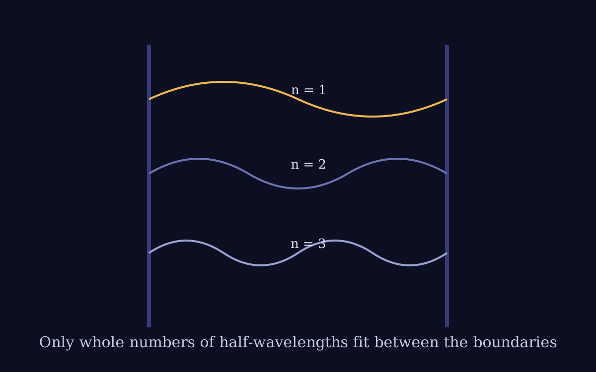
Change a one-dimensional cavity, field mass, selected mode, and mode cutoff. Each normal mode behaves like an oscillator, while an absolute zero-point sum remains regulator- and renormalization-dependent.
Selected ℏω: 0.620 eV
Selected ½ℏω: 0.310 eV
Cutoff N: 10
Σ½ℏω through N: 1.705e+1 eV
Increasing the cutoff increases this bare finite-mode sum. That sensitivity is a renormalization problem, not evidence that the displayed total is an accessible battery or a demonstrated work cycle.
This one-dimensional free-field cavity omits polarization, transverse geometry, interactions, material response, and the renormalization condition that defines an observable comparison.
Level 4 · Advanced undergraduate teaching kit
Record the investigation. Teach the reasoning.
A learner-facing lab record and a course-specific instructor guide turn the live model into a repeatable classroom investigation.
Learner record
Field-mode cutoff and observable-difference study
How do cavity geometry, mode cutoff, and subtraction choice affect raw vacuum sums and observable differences?
Download learner recordInstructor guide
Teach for evidence, not button pushing
Learners distinguish quantized mode spectra, regulated formal sums, renormalized parameters, and operationally defined observables.
Download instructor guideLesson 1 of 3
From classical fields to quanta
Why does each field mode behave like a quantum harmonic oscillator?
A classical field has a value at every point, and its action yields a partial differential equation. Fourier decomposition turns a free field into independent normal modes.
Canonical quantization promotes mode amplitudes and momenta to operators. Creation and annihilation operators organize the Fock-space spectrum; a particle is an excitation relative to a chosen state and mode basis.
Worked example
What is the energy spectrum of one free bosonic mode of frequency ω?
- 1. Map the mode to a harmonic oscillator.
- 2. Introduce number operator N=a†a.
- 3. Use H=ℏω(N+½).
- 4. Apply N|n⟩=n|n⟩.
E_n=ℏω(n+½).
Try it
Mode-counting laboratory
Materials: String, cavity, or numerical eigenvalue solver
- 1. Specify boundary conditions.
- 2. Find allowed wave numbers.
- 3. Convert them to frequencies.
- 4. Track how the spectrum changes with geometry.
Notice: The state and allowed modes depend on both the field equation and the physical boundary model.
Check your understanding: Is the vacuum the same particle state for every observer and spacetime?
Answer: Not always.
Particle and vacuum definitions can depend on the choice of time evolution, observer, or background.
Lesson 2 of 3
Propagators, interactions, and amplitudes
What do diagrams calculate, and what should not be read literally from them?
A propagator is a Green function encoding how disturbances correlate between spacetime points. Interactions generate perturbative corrections organized by powers of a coupling.
Feynman diagrams are terms in an expansion of an amplitude. Internal lines are not directly observed particles following hidden trajectories; measurable predictions emerge after amplitudes are combined into probabilities or cross sections.
Worked example
Why can two amplitudes interfere before probabilities are computed?
- 1. Identify indistinguishable alternatives.
- 2. Add complex amplitudes.
- 3. Take the modulus squared.
- 4. Retain cross terms.
|A₁+A₂|² contains interference terms 2Re(A₁A₂*).
Try it
Diagram-to-observable ledger
Materials: A simple tree-level scattering example
- 1. Label external states.
- 2. Write conservation at each vertex.
- 3. Identify coupling order.
- 4. State the cross section or rate the amplitude supports.
Notice: The observable sits at the end of a calculation chain, not inside a diagram's visual metaphor.
Check your understanding: Are virtual particles directly detected intermediate objects?
Answer: No.
They are internal elements of a perturbative representation and can depend on gauge or calculation scheme.
Lesson 3 of 3
Renormalization and observable vacuum effects
Which infinite expressions are artifacts of description, and which differences survive as measurements?
Loop and zero-point expressions require a regulator. Renormalization absorbs scheme-dependent pieces into measured parameters while leaving scale-dependent predictions for observables.
Vacuum-dependent phenomena such as Lamb shifts and Casimir forces concern differences, response functions, and specified boundary/material systems. A formal absolute sum does not by itself define extractable net energy.
Worked example
Why does subtracting two mode spectra require a shared physical prescription?
- 1. Regulate both spectra consistently.
- 2. Match high-frequency material behavior and geometry.
- 3. Subtract before removing the regulator.
- 4. Relate the finite remainder to a force or energy difference.
A finite prediction is meaningful only within the stated model and renormalization conditions.
Try it
Claim-boundary classification
Materials: Short excerpts about vacuum energy
- 1. Mark formal quantities.
- 2. Mark renormalized parameters.
- 3. Mark measured differences.
- 4. Identify any unsupported conversion to usable work.
Notice: The word vacuum can refer to a state, a renormalization convention, or an experimental configuration; they are not interchangeable.
Check your understanding: Does the term ½ℏω for every mode prove a device can draw continuous net work from the ground state?
Answer: No.
A work cycle, coupling, backreaction, and complete energy accounting are additional physical requirements.
Formula-to-meaning deck
Read the equation in ordinary language.
ℒ=½∂_μφ∂^μφ−½m²φ²
A free scalar-field Lagrangian determines propagation and mass.
φ(x)=∫d³k/[√((2π)³2ω_k)](a_ke^{-ikx}+a†_ke^{ikx})
The quantum field is expanded into annihilation and creation modes.
⟨0|Tφ(x)φ(y)|0⟩=D_F(x−y)
The time-ordered two-point function is the Feynman propagator.
Independent practice
Problem set
Work each problem before opening its hint and solution.
1. For ω_k=√(k²+m²) in units c=ℏ=1, what is the massless dispersion?
Reveal hint
Set m=0.
Reveal solution
ω_k=|k|.
2. What coupling order is a diagram with two interaction vertices each proportional to g?
Reveal hint
Multiply vertex factors.
Reveal solution
Order g² in the amplitude.
3. Why must a cutoff-dependent bare parameter not be reported as an observable?
Reveal hint
Consider what is fixed by experiment after renormalization.
Reveal solution
Its value depends on the regulator and scheme; only renormalized predictions tied to measurements are physical.
Derivation studio
Build the result, line by line.
Keep the assumptions visible so the mathematics remains auditable.
Starting point
Free-field mode oscillator
S=∫d⁴x[½φ̇²−½(∇φ)²−½m²φ²]
- 1. Fourier expand φ in spatial modes.
- 2. Use orthogonality to remove cross terms.
- 3. Identify one coordinate q_k per mode.
- 4. Read each term as an oscillator with ω_k²=k²+m².
H=Σ_k½(|p_k|²+ω_k²|q_k|²)
Free-field quantization inherits the oscillator ground state mode by mode.
Starting point
Klein–Gordon propagator equation
(□+m²)φ=J
- 1. Define a Green function D satisfying the sourced operator equation.
- 2. Fourier transform spacetime derivatives.
- 3. Solve algebraically in momentum space with a pole prescription.
- 4. Transform back to spacetime.
(□+m²)D_F(x−y)=−iδ⁴(x−y)
The propagator is an inverse differential operator with boundary conditions, not a classical path.
Computational notebook
Turn the model into an experiment.
Scalar-field modes and correlators
How do lattice size, spacing, mass, and boundary conditions alter a free field's spectrum and two-point correlation?
Inputs
- • One-dimensional lattice size and spacing
- • Field mass
- • Periodic or fixed boundaries
Algorithm
- 1. Build the discrete Laplacian.
- 2. Diagonalize normal modes.
- 3. Construct the regulated equal-time correlator.
- 4. Vary cutoff and finite volume separately.
Evidence to produce
- • Mode spectrum
- • Correlation versus separation
- • Cutoff and finite-size sensitivity analysis
Paper-reading studio
Interrogate the source, not its reputation.
Reconstruct the assumptions, reproduce one calculation, and stop at the boundary of the reported evidence.
Vacuum-claim reconstruction
Is the source calculating an absolute formal term, a renormalized difference, a response, or a measured observable?
- 1. State the field, state, and boundary conditions.
- 2. Identify regulator and renormalization prescription.
- 3. Locate the operational observable.
- 4. Audit any step from fluctuation to net work.
Calculation to reproduce: Reproduce one regulated mode sum, two-point function, or lowest-order amplitude using the source's assumptions.
Evidence boundary: Quantum vacuum effects are established, while a self-sustaining vacuum-energy extraction cycle requires separate demonstrated dynamics and energy accounting.
Continue into the evidence
Source-linked next reading
Lecture 7: QFT and the vacuum
Modes, ground states, measured vacuum phenomena, and unresolved absolute-energy questions.
Chapter 2: Vacuum energy and the ZPF
Trace standard equations and competing interpretations without merging their evidence status.
Lecture 8: Casimir effect measured
A boundary-dependent observable with real material and metrology corrections.